Abstract
The theoretical groundwork in a previous paper [1] showed how selective grounding improvements can be used to reduce undesirable voltages on grounded conductors. A field effort was engineered based on that work. Grounding was improved at a number of taps to reduce interference voltage being experienced on a cluster of power distribution systems in Michigan. In this follow-up paper, the findings of this application effort are compared to the theorized results predicted in the previous paper, and the cost effectiveness of grounding efforts is examined. Much more is also learned about the practical aspects of grounding improvements on electrical utility systems.
Introduction
Construction codes and industry specifications provide a safety net of rules and guidelines, but on occasion the conditions are such that special measures have to be taken that go beyond the standard requirements. Improvement of the electrical grounding on utility distribution plants and at other industrial or commercial facilities is an engineering consideration that comes up after the facilities are built, often as a result of a safety or interference problem [1-3]. For example, concerns over stray voltage have induced states such as Wisconsin to step up the grounding requirements for electrical distribution systems above the requirements set by the National Electric Safety Code, by requiring a ground rod at every pole in rural areas.
A previous paper [1] outlined an analytical approach to study the effects of improving the grounding selectively. It showed that a lattice network can be used to model the grounded conductor of a distribution line in the presence of interference signals and other line conditions. The model can be used to experiment with the extent and location of grounding improvements. For example, one objective may be to reduce the neutral voltages along the whole line, because of poor earth conductivity; another may be to decrease interference voltage at line ends.
The analytical approach with grounding improvements is more effective and much less costly than trial experimentation. The modeling can be used to identify the grounding improvements in terms of location and amount that are sufficient to resolve a problem, and optimize the solution for the lowest possible cost. The analytical approach can show whether the goals are achievable at all and at what price, before a shovelful of soil is even moved. More importantly, it helps to avoid costly mistakes, because the grounds are not easily removed once they are installed.
This paper outlines and analyzes a grounding improvement that was based on this approach and the results of the previous paper [1]. A real application of these principles provides experience and evidence for the validity and usefulness of this engineering approach, and also provides valuable information on practical construction approaches and problems. Most importantly, this paper provides cost-effectiveness information, which is just as important for engineering as the modeling tool because of the uncertainty associated with grounding efforts.
Background
The first paper outlined the effects of improving grounding locally or uniformly along a power distribution line, at different levels of improvement, and in the presence of various types of interferences. A resistive lattice was shown to be simple and accurate enough for computer modeling of the line grounded conductor: the modeling can be done in a spreadsheet. It was shown that improving grounding is most effective as a technique when the earth has a very high resistivity. The dynamics of the phenomenon were compared to the movements on a balancing scale. The distribution neutral voltages have a minimum which is referred to as the fulcrum, and as grounding improvements cause voltages to drop on one side of the fulcrum, they cause voltages to rise on the other side of the fulcrum, although not in a linear fashion.
The interference source has an effect on the voltage distribution and the way neutral voltages respond to grounding improvements [2-6]. Interference swells and tail-end voltage rises are most sensitive to grounding improvements. Improving grounding only at the ends of a distribution line can be very cost-effective as a first step, followed by uniform grounding improvements along the line if more voltage reduction is needed.
The most intriguing finding, however, was that the greatest effect on a voltage problem can be achieved by grounding improvement treatment at the last dozen poles of the line. This is illustrated in the neutral voltage reduction curves as a function of the number of poles treated at the line end, which is reproduced here in Figure 1. This concept was capitalized on in designing measures to reduce interference voltages in a real situation by two power companies in Michigan: Upper Peninsula Power Company (UPPCO) and Wisconsin Electric Power company (WEPCo).
Job Description
A special radio communications system [2, 3] operating near the power frequency and utilizing earth as the return path for current, causes small voltages to be induced on a number of power distribution facilities in its immediate vicinity. These voltages on the neutral line conductor represent a nuisance and a potential safety concern. At some distance from this source, the interference is of a marginal concern and located mostly at the end of taps. One proposal was to improve the grounding at these locations to lower the interference voltages enough so that they would not be a concern, and thus require no further interference mitigation work.
Two companies with interference on their plants undertook such efforts with construction funds provided on a reimbursement basis from the communications system. A number of taps in the marginal interference areas were identified (see Table 1) where the interference voltage on the distribution line neutral could be lowered below the level of concern with improvements in grounding. The work affected 22 separate taps, dispersed over five rural distribution circuits, clustered at a dozen noncontiguous locations in a sparsely populated area of 600 square miles.
| Company-Substation | Location | Range, Township, Sections |
Number of Poles |
Number of Spans |
Taps |
|---|---|---|---|---|---|
| UPPCO-Barnum | CR-PNA | 27, 47, 30 | 5 | 7 | 1 |
| UPPCO-Barnum | CR-PL | 27, 47, 29-30 | 17 | 37 | 1 |
| UPPCO-Gwinn | CR-MS | 26, 46, 26 | 7 | 11 | 1 |
| UPPCO-Gwinn | Shag Lake | 26, 45, 24-26 | 15 | 31 | 1 |
| UPPCO-Gwinn | M35 | 26, 45, 13 | 8 | 13 | 1 |
| UPPCO-Perch Lke | CR-LY | 30, 46, 26/35 | 3 | 13 | 1 |
| UPPCO-Perch Lake | CR-LLN | 29, 46, 31 | 4 | 9 | 1 |
| UPPCO-Perch Lke | S. Rep. | 29, 46, 30 | 25 | 57 | 3 |
| UPPCO-Perch Lake | CR-LLL | 29, 46, 19 | 7 | 7 | 1 |
| UPPCO-Perch Lake | CR-LO | 30, 46, 25 | 10 | 19 | 1 |
| UPPCO-Perch Lake | S. Rep. | 29, 46, 18 | 16 | 30 | 1 |
| UPPCO-Perch Lake | Sub | 29, 46, 06/08 | 13 | 22 | 1 |
| UPPCO-Perch Lake | Michigamme. R. | 30, 45, 36 | 7 | 14 | 1 |
| WEPCo-Felch | CR-426 | 28,43,24 | 15 | 27 | 1 |
| WEPCo-Felch | CR-581 | 28, 43, 14 | 14 | 24 | 1 |
| WEPCo-Felch | Turner Rd. | 28, 43, 22 | 12 | 19 | 1 |
| WEPCo-Felch | Cootware Rd. | 28, 43, 36 | 21 | 38 | 2 |
| WEPCo-Greenstone | CR-601/478 | 29, 47, 28 | 24 | 49 | 2 |
| Totals | 223 | 427 | 22 | ||
A dozen poles were identified at the end of each tap, in accordance with the findings of the paper [1]. The taps were not all ideal and monotonic straight lines; many of them had spurs of a few spans and zig-zagged along roadsides. The design engineer used the dozen-poles guideline in selecting manually the poles to be treated from line maps augmented with interference voltage data. The series of poles to be treated were not contiguous, and transformer poles were excluded to avoid complications. In the end, the number of poles treated on each tap varied from a minimum of 3 to a maximum of 16, with an average of 10 poles per tap. As it turned out, the number of treated poles were mixed with just as many untreated poles, making the average length of treated tap 19 spans long.
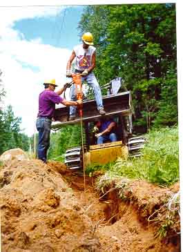
Deep grounding was chosen as the preferable technique for grounding improvement because of the better results compared to the use of counterpoise in this area where the earth has poor conductivity. Deep grounding refers to the installation of long ground rods deep below the surface. This is achieved by coupling standard 8-ft ground rods, as they are installed, one after another and one at a time, typically until a point is reached at which the rod will not penetrate further. This technique is especially effective in areas of poor earth conductivity, because if the deep rod reaches into the water table, a much lower resistance to earth is achieved notwithstanding the poor earth conductivity at the surface.
Various construction standards were developed around this grounding improvement theme. The main distinction was whether the deep ground rod was installed at the base of the pole or some distance away from the pole. Figure 2 shows the construction standard developed for installing the deep ground rod 16 ft away from the pole. The objective was to keep to a minimum the coupling between the existing rod at the base of the pole and the new deep ground rod, to obtain the most benefit from the finished construction. However, it was unknown beforehand how deep the ground rod would be at any particular site. The distance away from a pole to install the deep ground rod was set at 16 ft, based on the rationale that the mutual coupling is minimized by keeping the separation between rods equal to the length of the longest rod [7], and the expectation that the average deep ground rod depth would be 16 ft, or two standard rod lengths. Furthermore, for budgetary cost considerations, no more than eight coupled 8-ft ground rod sections could be installed at a site, and no more than two attempts could be made at a pole to install a deep ground rod in case of surface rock. The average depth for the deep ground rod turned out to be 30 ft, and a more optimal distance for locating the deep ground rod would have been 30 ft from the pole.
Outside of these guidelines, the companies were free to decide in the field how to improve the grounding at a pole. The company could choose to utilize the existing rod at the base of the pole and add more to it, turning the existing rod into a deep grounding rod. Alternatively, the company could install a new deep ground rod 16 ft away from the pole and run a buried, bare, copper wire to bond the new rod to the existing one at the base of the pole (see Figure 3). In those few cases where there was no ground rod at the pole, one was installed, together with the pole grounding wire.
To record the grounding improvements, the construction crew was asked to measure the pole grounding resistance upon reaching the site and before doing any modification. The measurement was repeated by the same crew immediately after the grounding improvement. This provided a measurement of the improvement of the grounding resistance at the pole. The resistance was measured using the AMC Ground Resistance Testers, Models No.3700, and 3730. The interference voltage on the line neutral conductor was measured by a separate crew by tapping onto the pole ground wire and using an earth reference test ground rod installed temporarily 50 ft from the pole and broadside to the line. The voltage measurement was done in the days immediately before and after the grounding work was performed for each tap, and provided a measurement of the effect of the grounding improvement on the interference voltage reduction. The separation between resistance and voltage measurements was necessary to measure the impact on the interference voltage due to grounding improvements along the whole tap, and not just the relative improvement at a single pole.
Results and Discussion
The two companies approached the job in different ways. UPPCO scheduled the job on days of slow activity in regular company work and dedicated a crew that usually consisted of two men but on occasion grew to four men. The job started in January 1997 and ended in the spring. This company chose to install most of the deep grounds at the base of the pole; only a handful were installed 16 ft away. WEPCo did the work in the summer of 1997 in just six days, with a field crew of 6 to 9 men, working on different sites at the same time. It installed all deep ground rods 16 ft away from the pole. It rented a backhoe to dig a trench to bury the connecting wire. Both companies utilized standard 8-ft ground rods attached to each other with compression couplers.
Table 2 is a summary of the work that was performed. Altogether 231 line poles were treated and 791 standard 8-ft rods were installed. The average depth of a ground rod was 30 ft. The deepest rod was 64 ft, the maximum allowed under the construction protocol, and occurred 10 times. There were cases also where the depth was just a few feet, because of rock present on the surface.
| UPPCO | WEPCo | Total | |
|---|---|---|---|
| Crew Size | 2-4 men | 6-9 men | |
| Performance Period | 5 months | 6 days | |
| Sites Treated | 148 | 83 | 231 |
| Labor Hours | 840 | 380 | 1220 |
| 8-ft Rod Sections | 543 | 248 | 791 |
| Average Depth of Rod | 34 ft | 24 ft | 30 ft |
| Average Labor per Site | 5.5 hr | 4.7 hr | 5.2 hr |
Table 3 is a summary of the statistical analysis of the data collected during this job. The data, as mentioned above, consist of ground rod resistance to earth and relative interference voltage to remote earth measured at each pole before and after the grounding improvement job. The data sample size varies because data were missed or lost or because of oversampling. The statistical analysis was carried out on the log-transform of the data, which provides a distribution that is closer to the standard normal distribution (see Figures 4 and 5).
| Zbefore | Zafter | Vbefore | Vafter | |
|---|---|---|---|---|
| Sample Size | 199 | 199 | 211 | 248 |
| Average | 258 | 78 | 2.1 V | 1.6 V |
| Average 95 Percentile Range | 222 - 299 | 65 - 93 | 1.9 - 2.3 V | 1.4 - 1.7 V |
| Sample 95 Percentile Range | 32 - 2,083 | 7 - 917 | 0.4 - 10.6 V | 0.4 - 6.6 V |
Table 3 indicates that the average pole grounding resistance was 258 before the treatment and dropped to 78 after the grounding improvement. This is a 3.3-fold improvement in pole conductivity to earth. The average interference voltage was 2.1 V before treatment and dropped to 1.6 V after the grounding improvement. This represents a 24% reduction on average in the interference voltage.
It is interesting to compare these results to the ones predicted in Figure 1. Using interpolation, the voltage drop at the end of line (Figure 1) corresponding to treatment at the last 10 poles of the line, with grounding improvement of 3.3-times, is about 15%. If the average number of spans affected by the treatment,19, is used on the ordinate axis of Figure 1 instead of the number of poles, the voltage drop is about 23%. This substitution is reasonable because the interference voltage affected by the grounding improvement is related to the number of spans and not the number of poles. Furthermore, little is known about the exact nature of the interference voltage, and Figure 1 shows curves between specific interference patterns to choose from. Another difference between the field results and the theorized ones to keep in mind is that the results presented here are statistical representations while the results discussed in the previous paper are deterministic results specific to a case. Also note the difference between voltage drop at the end of a line in the theoretical analysis [1], and the average pole interference voltage drop in the field data analysis. Notwithstanding all these differences, there seems to be considerable agreement between the theoretical analysis and the field findings. Actually, the field findings seem to indicate that the benefits in interference voltage drop may be at least what was predictable, and maybe better.
Figure 4 outlines the distribution of the pole grounding resistance before and after the grounding improvements. It clearly shows a drop overall in pole grounding resistance, which is supported by the data in Table 3. The drop in the samples average is not a sample fluke, but a statistical fact, as shown in Figure 4, which is not surprising considering the clear-cut nature of the resistance data. Figure 4 shows the before-improvement grounding resistance distribution curve to roll off rapidly to zero at around 1,200 . This is because the AMC meter Model 3730 has a maximum range of 1,200 . There were therefore many measurements that pegged at 1,200 , and were recorded as such, even though it was clear that the grounding resistance was much higher. This suggests that the actual grounding improvement is higher that has been calculated. Note also that following the grounding improvement job, hardly any instances are recorded with a grounding resistance above 1,200 .
Figure 5 similarly outlines the distribution of the pole interference voltage before and after the grounding improvements. It clearly shows a shift of the overall distribution, toward lower voltages, with the grounding improvements. The drop, however, is not as marked as the one observed in Figure 4. The expected probability range (95%) of the sample averages in Table 3, shows clearly that the drop is not merely a statistical fluke, but a real effect. Figure 5 shows, more importantly, a drop in cases of high pole interference voltage. For example, the number of poles with interference voltage of 5 V or higher drops from 14% before treatment to 6% after grounding improvement treatment.
Returning to Table 2, we can appraise the cost of this job and consequently obtain the cost for the reported benefits. The material used in this job (ground rods, couplers, wire, and connectors) is of relatively little value and an easy-to-handle variable that can be pegged as a constant for the average site. The cost of transportation, vehicles, and equipment, can be pegged to the labor hours, because of the ordinary nature of this job. Labor thus constitutes the main cost component. Knowing the labor that is required on average to improve the grounding at a site, it becomes a relatively simple calculation to figure out the cost in dollars (multiply labor hours by labor rates, add overheads, use appropriate multiplier or rates based on labor hours to figure transportation and equipment usage, add material and any additional charges and fee depending on the company). Labor hours is therefore used here as a normalized scale of cost.
Table 2 shows that the cost of each pole grounding improvements based on labor hours is 5.2 manhours. The results and performance turned out to be remarkably similar between the two companies. The differences were related to the different approach taken by each company, the different size of the jobs, the different time when each company did the work, and the difference in soil encountered by each company that affected the depth of the rod. The average depth of the UPPCO ground rod was 34 ft versus 24 ft for WEPCo. Furthermore, UPPCO did most of the work in winter conditions, which is known to be a cause of slower performance. It had to clear the snow at the base of a pole and fight ground frost, a reason for doing most of the installations at the base of the pole. WEPCo did the work during summer, using larger crews, but it had to dig a 16 ft long trench at every pole to bury the connecting conductor.
The cost for a 3.3-fold improvement in grounding conductance at a pole is about 5.2 manhours of labor on average. The cost has been estimated to be about $450 pe site on average. The benefit of grounding improvement is a 23% reduction overall in the interference voltage.
Conclusions
The question of grounding improvement, often an afterthought in response to problems, has been addressed systematically in these two papers. The first one laid out a theoretical treatment, outlining the means to engineer solutions tailored to a specific situation. Some generic conclusions were derived in that paper by looking at typical problems and seeking cost-effective solutions.
This paper has reviewed a field effort that was based on that theoretical background to reduce an interference voltage problem. The effort has been very informative. Although not specifically designed so, the effort has provided a variety of situations and circumstances that make this effort very useful. Two different companies were involved, each pursuing its own approach within a set of ground rules. One chose to do the job slowly during periods of slack time, over many winter months, installing the deep ground rod at the base of the pole; the other company chose to do the job all at once in the summer, using a large crew, and installing the deep ground rod 16 ft away from the pole. The results were very similar.
Overall 231 pole were treated, affecting 22 taps dispersed over a wide area. The average ground rod depth was 30 ft, although many went down to the prescribed cap of 64 ft. Statistically we found that the pole ground conductance to earth was improved 3.3-fold on average, and this caused the overall interference voltage to drop by 23% on average. The labor for the installation of deep ground rods was 5.2 manhours per site on average.
The job provided somewhat better results than what had been predicted and was in line with the theoretical groundwork. Much more was learned on the practical side in planning and performing such jobs. The data contain much more information that will require further analysis and investigations. There are questions about the aging of the deep ground rods as the disturbed earth settles around them, and whether deep ground rods are indeed a more effective way of utilizing ground conductors vis-a-vis other systems such as counterpoises.
Acknowledgments
The authors express their appreciation to the Department of the Navy, which provided the opportunity to obtain the data, and to the power companies that cooperated in this effort, UPPCO and WEPCo.
References